 For several years, the genome-wide association study (GWAS) has served as the flagship discovery tool for genetic research, especially in the arena of common diseases. The wide availability and low cost of high-density SNP arrays made it possible to genotype 500,000 or so informative SNPs in thousands of samples. These studies spurred development of tools and pipelines for managing large-scale GWAS, and thus far they’ve revealed hundreds of new genetic associations.
As we all know, the cost of DNA sequencing has plummeted. Now it’s possible to do targeted, exome, or even whole-genome sequencing in cohorts large enough to power GWAS analyses. While we can leverage many of the same tools and approaches developed for SNP array-based GWAS, the sequencing data comes with some very important differences.
1. There Will Be Missingness
SNP arrays are wonderful tools that typically deliver call rates (the fraction of genotypes reported) of 98-99%. Sequencing, in contrast, often varies from sample to sample in read depth and genotype quality for many, many positions.
Targeted sequencing, including exome sequencing, tends to have a variable “shoulder effect” in which the read depth obtained forms a bell curve centered on each targeted region.
Thus, you get lower coverage outside of your target. Sometimes it’s enough to call variants, sometimes not. Polymorphic sites in such regions might only be called in 20% of samples, and this phenomenon is usually exacerbated by batch effects.
2. You Must Backfill Your VCF
The variant calls from next-gen sequencing are typically exchanged in VCF file format. Most variant detection tools output directly into that format, and most downstream annotation/analysis tools will read it. Importantly, variant callers typically don’t report positions that are wild-type. Otherwise the files would be huge.
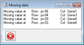
It’s quite easy to take VCF files from many different samples and merge them together. VCFtools will do that for you. Here’s the problem: unless the VCFs have information about every position (including non-variant ones), any variants called in sample 1 but not sample 2 will have the “missing data” genotype in the merged VCF file.
To illustrate with a very basic example, two samples each with three heterozygous SNPs:
VCF for sample 1:
CHROM	POSN	REF	ALT	...	SAMPLE1
chr1	2004	A	G	...	0/1
chr1	5006	C	T	...	0/1
chr1	8848	T	A	...	0/1

VCF for sample 2
CHROM	POSN	REF	ALT	...	SAMPLE1
chr1	2004	A	G	...	0/1
chr1	4823	G	A	...	0/1
chr1	8848	T	A	...	0/1

Merged VCF:
CHROM	POSN	REF	ALT	...	SAMPLE1	SAMPLE2
chr1	2004	A	G	...	0/1	0/1
chr1	4823	G	A	...	./.	0/1
chr1	5006	C	T	...	0/1	./.
chr1	8848	T	A	...	0/1	0/1
Now you can see the issue. We don’t know if site 4823 in sample 1 was wild-type or simply not callable in the sequencing data. Same deal for position 5006 in sample 2. And, because of reality #1, you can’t simply guess here. You truly need to go back to the BAM file for each sample and make a consensus genotype call for each missing genotype. Our center has a pipeline for doing this in every cross-sample VCF we produce, but I’m guessing that many sequencing service providers do not.
3. Batch Effects Are Guaranteed
Next-gen sequencing is a rapidly evolving technology. Sure, one platform dominates the market, but it also comes in many different forms: GAIIx, HiSeq2000, HiSeq2500, MiSeq, HiSeq X Ten.
 Even with one instrument, the reagent kits, software version, and run quality will affect the resulting sequencing data. Because a well-powered GWAS will require thousands of samples, the sequencing probably take long enough for something to change. There are other sources of variability, too:
- Library protocol (insert size, selection method, enzyme choice)
- Capture reagents. (manufacturer, version, probe type)
- Sequencing software version
- Aligner version and parameters
If I had to pick one thing to keep the same, I’d go with the reagent used for exome sequencing. There is no universally-accepted definition of the exome, and the hybridization capture technologies offered by leading vendors (Agilent, Nimblegen, Illumina) have key differences.
4. Expect Many Rare Variants
The genetic variants interrogated by most high-density SNP arrays are exceptional in a number of ways:
- Most are common with allele frequencies >1% in human populations.
- Most are found in multiple populations (European, African, Asian)
- Most are not in coding regions (the exome-chips address this somewhat).
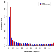
Casals et al, PLoS Genetics 2013
In other words, the SNPs chosen for inclusion on commercial arrays are the best of the best: high-frequency SNPs that represent, or “tag”, the variation for a much larger region. They must be informative, since a typical array tests about 600,000 SNPs, and a typical genome harbors over 3 million.
In contrast, sequencing will reveal variants across the entire allele frequency spectrum. Most of the variants won’t even be on a commercial SNP array, and 5% or so won’t even be in dbSNP. Thus, the allele frequency spectrum is dramatically different in a sequencing study. This will affect the analysis.
5. Expect Many Ugly Variants
Another requirement for inclusion on a high-density SNP array is assayability. The genotyping technologies are best suited to bi-allelic variants in unique (non-repetitive) regions of the genome. Highly variable sequences (i.e. high density of SNPs or other variants) can alter the assay, so they’re usually avoided.
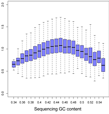
It is not fair to say that sequencing is completely unbiased by comparison, because probe selection (for targeted/exome studies) must consider properties like uniqueness and GC content. Read mapping, too, introduces bias. Even so, sequencing picks up a lot of the “ugly” variants that SNP arrays so meticulously avoid: low-complexity regions, indels, triallelic SNPs, tandem repeats, etc.
A multi-sample VCF can get pretty ugly. You might have a 2-base insertion right near a 3-base deletion with a SNP between them. You might see all four nucleotides at one SNP.
6. Not All VCFs Are Created Equal
Even VCFs which have been properly backfilled may differ slightly in form without breaking the format’s rules. That’s because the VCF specification allows some flexibility in the names of INFO and genotype fields, and what they contain. A minimalist VCF might contain genotypes with quality scores, whereas a fuller VCF could have 10-12 fields (genotype, score, depth, read counts, probabilities, filter status, strand representation) for every single genotype.
It will be important to find the right balance of keeping enough information while maintaining reasonable file sizes. Also, some VCFs will include genotypes that have been failed by a filter or QC check, and that failure may only be noted in the FT field of the genotype (note in the FILTER column). If your analyst or conversion tool isn’t aware of this, you could be pulling in a lot of bad calls.
7. Variant QC Is An Art Form
The genotype table from a GWAS is a beautiful thing. It has 600,000 or so rows, one column for every sample, and 99% of those cells have a good, clean genotype. With PLINK or any number of tools, it’s easy to zip through the table and remove the variants with missingness or Hardy-Weinberg problems.
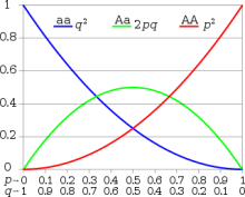
Hardy-Weinberg equilibrium
With sequencing data, one can and should still use these metrics in a dataset. But if you removed variants outside of Hardy-Weinberg equilibrium, you probably won’t have many left. Genotyping accuracy in NGS is a different ball game than SNP arrays. With sequencing it is usually quite accurate, but the accuracy isn’t constant: it’s controlled by sequencing depth and other factors. The careful heterozygote/homozygote balance prescribed by nature can shift quite easily.
There are other confounding factors, too. We recently examined ten randomly-selected Hardy-Weinberg outliers from a sequencing dataset. Three proved to be dinucleotide polymorphisms (DNPs), another couple were in close proximity to common indels (causing artifactual calls), a few were in highly repetitive sequences, and at least one seemed perfectly sound. By “sound” I mean that when I pulled up the variant calls in IGV, they looked good.
Deciding where to draw the line and include or exclude variants is not a quick and easy decision.
8. Massive Computational Burdens
This last reality isn’t surprising at all: the computational burden is huge. Because sequencing studies uncover most variants within their targets, and those variants tend to be rare, the genotype table (variants in rows, samples in columns) even for exome studies is huge.
 The hard disk required for data storage, and the resources (memory, CPU) required for data manipulation/analysis dwarfs what’s required for SNP array data. That’s why some groups, such as our colleagues at Baylor’s Human Genome Sequencing Center, are turning to cloud computing.
The real bummer about the already-considerable computational load is this: if a sample is added to the study, it will undoubtedly contribute some new variants, which means that the entire genotype table must be re-calculated. For example, an exome study with 1,000 samples might have 60,000 variants. That’s already 60 million cells. When you add sample 1001, it might have 500 variants not seen in other samples. To “backfill” the genotypes adds half a million backfill operations, just to add one sample.
You can imagine how this begins to snowball. Finalizing the sample set before running analysis has never been more important.
On the Bright Side
These caveats of the sequencing GWAS, while important, should not detract from the advantages over SNP array-based experiments. Sequencing studies enable the discovery, characterization, and association of many forms of sequence variation — SNPs, DNPs, indels, etc. — in a single experiment. They capture known as well as unknown variants.
Sequencing also produces an archive that can be revisited and re-analyzed in the future. That’s why submitting BAM files and good clinical data to public repositories — like dbGaP — is so important. Single analyses and meta-analyses of sequencing GWAS may ultimately help us understand the contribution of all forms of genetic variation (common, rare, SNPs, indels) to important human traits.
Great post, thank you very much.
In point 4 you said that, when sequencing, you expect to find about 5% new variants that are not in dbSNP. Where do you get this estimate from? Do you know any good literature for this estimate?
Thanks!
One crucial element beyond rare variants.
Sequenced genomes will contain very private variants, including completely novel portions of genome sequence as shown first by Michael Snyder in his paper.
This could have fundamental real consequences (even containing entire genes) but none of us, currently take them int ou account in our routine…
Thanks for the great post Dan!